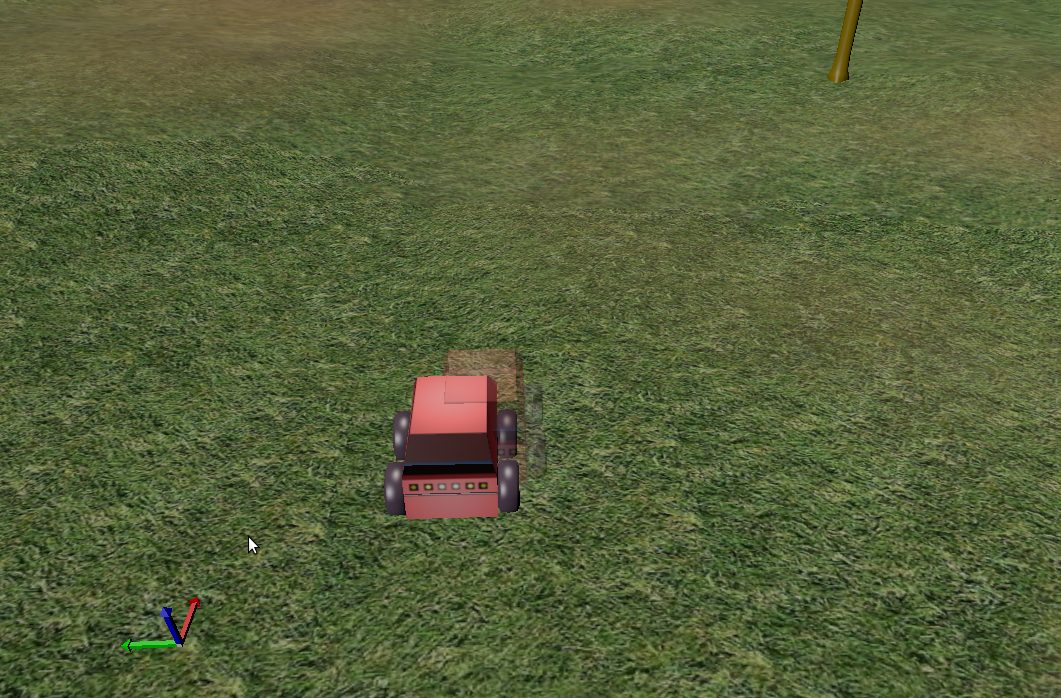
Noise and ghost tutorial builder pymorse
This tutorial will show how to add and configure noise modifiers
to your components, and will illustrate the use of ghost robots.

Pre-requisites
- You must have completed the first tutorial.
- We recommed that you also complete the cat and mouse tutorial.
Creating the scenario
We’ll use the Builder API to configure the scenario’s robots. First we will configure the real ATRV robot.
Create a new ATRV robot:
from morse.builder import *

robot = ATRV()
We will add a pose sensor to it, and make the data available through the socket interface:
pose = Pose()
robot.append(pose)
pose.add_stream('socket')
Next we make it controllable by the keyboard, using the correct actuator:
keyboard = Keyboard()
robot.append(keyboard)
Finally we alter the initial pose data with some Gaussian noise:
pose.alter('Noise', pos_std=.5, rot_std=0, _2D=True)
Note
The noise parameters are documented in the Noise modifier.
Now we’ll create the ghost robot: it is intended to represent some external computation, without conflicting with the simulated robots.
Create another ATRV robot, the ghost:
ghost = ATRV()
Next we add a Teleport actuator to control it:
teleport = Teleport()
ghost.append(teleport)
Finally, we make the robot a ghost, and add the socket interface to it:
ghost.make_ghost()
ghost.add_default_interface('socket')
And finally we complete the scene configuration:
env = Environment('land-1/trees')
env.create()
The complete script can be found at: $MORSE_SRC/examples/tutorials/noise_ghost_tutorial.py.
Ghost is noise script
As a very simple example of how to use the ghost robot, we’ll create a Python script to connect to MORSE and display the noisy position:
import pymorse

with pymorse.Morse() as morse:
  while True:
    pose = morse.robot.pose.get()
    morse.ghost.teleport.publish(pose)
    morse.sleep(.1)
The whole program can be found at: $MORSE_SRC/examples/clients/atrv/ghost_noise_script.py
Run morse with the builder script to create the scenario. You will be able to control the robot with the arrow keys on the keyboard:
$ cd $MORSE_SRC/examples/tutorials
$ morse run noise_ghost_tutorial.py
Then run the Python noise display script from another terminal. The ghost position will show the noisy robot position as altered by the Noise modifier.:
$ cd $MORSE_SRC/examples/clients/atrv
$ python3 ghost_noise_script.py
Ghost is filtered script
Using the ghost robot to show the noise applied to the position data isn’t very interesting. In this script, we will see how we can use the ghost to display more useful information, for instance the robot position estimated from the noisy position.
For this script, you need to install the numpy and scipy python packages:
$ sudo apt-get install python3-numpy python3-scipy
or:
$ sudo easy_install3 numpy scipy
The whole program can be found at: $MORSE_SRC/examples/clients/atrv/ghost_estimation_script.py
It differs from the previous one in that the robot position is estimated from the robot’s measured noisy position, by using an unknown input Kalman filter. To this end, a very simple extended autonomous state-space dynamic model of the robot has been considered:
X_{ext} &= \begin{pmatrix} x & ux & y & uy\end{pmatrix}^T \\ A_{ext} &= \begin{pmatrix} 0 & 1 & 0 & 0\\ 0 & 0 & 0 & 0\\ 0 & 0 & 0 & 1\\ 0 & 0 & 0 & 0 \end{pmatrix}\\ \dot{X}_{ext} &= A_{ext} * X_{ext}
where x, ux, y, uy are the position and control variables along the
x and y axes.
The robot’s x-y positions are subject to a white Gaussian noise (with zero mean). Thus,
following the dynamic model notations, the measured vector is
Y_{meas} &= C_{ext} * X_{ext} + w \\ C_{ext} &= \begin{pmatrix}1 & 0 & 0 & 0\\ 0 & 0 & 1 & 0\end{pmatrix}
where w stands for the white noise.
Grounded on the above model, the derivation of the Kalman filer is obtained by solving
the following Riccati equation, using the solve_continuous_are function,
where, the symmetric matrices Q and R are the design variables providing the confidence we
have in the measurement and the model (typically, the trade-off is adjusted by tuning the ratio Q/R,
available in the script through the measure_confidence variable).
The solution of the Riccati equation is then used to compute the Kalman gain L as follows:
L = P * C_{ext}^T * (R / I)
The discrete-time Kalman observer state-space matrices are simply obtained using a backward discretization:
A &= I + (A_{ext} - L * C_{ext}) * dt\\ B &= L * dt\\ C &= C_{ext}
where dt is the discretization period.
To run it, just launch this script instead of the previous one:
$ python3 ghost_estimation_script.py
